Visualizing the Concept of Spatial Coherence - The Double Slit Experiment with Incoherent and Coherent Light
What happens when the double slit experiment is performed with spatially incoherent light (for example, with a light bulb)? And how does it differ when it is performed with coherent light (for example, with a laser)?
The surface of a spatially incoherent light source can be represented by a collection of randomly emitting electric dipoles, for example, the atoms experimenting radiative transitions in the filament of a light bulb. The light source may actually be near monochromatic like a low pressure sodium discharge lamp (dominated by the bright doublet known as the Sodium D-lines at 588.99 and 589.59 nanometers), but ultimately the field exiting the incoherent light source involves a small spectrum of wavelengths and randomly changing phase in time. Unlike the interference features produced by a laser light source, that can be seen, for example as a speckle pattern, the interferences produced by incoherent source, are not stationary but change rapidly, so they are "averaged out" by a sensor, like an human eye responding to the time-averaged squared magnitude of the field. How much the interference artifacts disappear will depend on the characteristics of light source and the sensor placement.
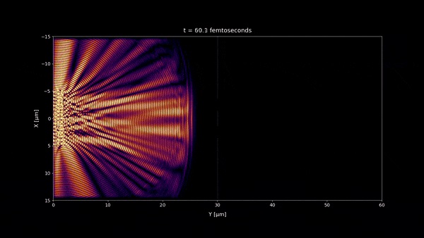
I thought that a visualization of the topic could be helpful, but I found almost zero of them in the literature. The main idea of this video is to illustrate and show the subtle details of the concept of coherence by means of three simulations of the light propagating through the double slit at different time scales: (femtoseconds, picoseconds, and microseconds) to show their differences.
The experiment demostrated in this video is a key result in statistical optics. It can also be mathematically treated with the Van Cittert-Zernike theorem and the concept of mutual coherence, that we'll discuss in the last two sections.
How I made the simulations:
The simulations were done using the finite-difference time-domain method (FDTD) applied to Maxwell equations.
The incoherent light is simulated by computing the field created by oscillating dipole sources with random phases and wavelengths and randomly placed inside the light source dimensions (a rectangle). The dipoles represent the radiative transitions of the excited atoms of the light source.
The microseconds and picoseconds simulations are obtained when the field is averaged over that period of time.
You can find the source code of the simulations in their GitHub repository.
You can change the parameters of the simulations just typing the values you want in the scripts that are indicated.
While the femtoseconds simulations only took a few minutes to be completed, the microsecond simulations 2:28 took hundreds of hours to be completed in a personal computer!
In the femtoseconds scale you can slow down the video to x0.25 in youtube settings if you find the flickering annoying. Also the video is uploaded at HD 1440p to avoid the artifacts that youtube video encoder creates with the waves at lower resolutions. You can see all fine details of the waves if you watch the video at this resolution.
Why do the interference patterns fluctuate on the picoseconds time scale?
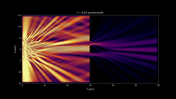
Interference patterns fluctuate on picoseconds time scale because this is the order of magnitude of the coherence time of the source. This is the minimum time to make the electric field change considerably [1].
\begin{equation} \tau_{coh} \approx \frac{ \lambda ^2}{c \Delta \lambda} \label{eq:1} \end{equation}
where:
$$ \Delta \lambda = \text{bandwidth of the light source}$$ $$ \lambda = \text{center wavelength}$$ $$ c = \text{speed of light}$$
In the simulation was used a wavelength of $ \lambda = 650 \text{ nm}$ and a bandwidth of $\Delta \lambda = 1 \text{ nm}$. Plugging these values in the formula \eqref{eq:1} we get a coherence time of:
$$\tau_{coh} \approx 1.4 \text{ picoseconds} $$
You can see that a very narrow bandwidth $ \Delta \lambda = 1 \text{ nm}$ is enough to make interferences fluctuate very fast. $ \lambda = 650 \text{ nm}$ correspond to red light, and the narrow bandwidth makes almost no difference in color to the human eye.
When the intensity is averaged over a few microseconds no fluctuations can be seen. This is the reason that although the wave-like behaviour of light, we don't usually see the interferences.
Further explanations:
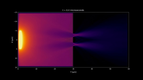
- In microseconds time scale 1:20 and any longer time scale, no incoherent light interference pattern should be visible as we observe in most of our daily life. But a stationary wave is still visible in the microseconds time scale near the double slit wall. However because its size is very small , you won't notice it at macroscopic scale and instead you will see a uniform pattern. (notice that the space scale of the simulations are 60 x 30 μm)
Mathematical description of the spatial coherence
For incoherent light, the time variations in field amplitude are statistical in nature, and only statistical concepts can provide a satisfactory description of the field. The theory of coherence is a vast topic that will not discuss here. The reader interested in a complete treatment can consult [1] [4] or [5]. Instead, here, we'll be limited to defining the basic concepts.
Consider the electric field $E(\mathbf{r}, t)$ evaluated in two different points $\mathbf{r_1}$ and $\mathbf{r_2}$. We define the mutual coherence function $\Gamma(\mathbf{r_1}, \mathbf{r_2}, \tau)$ between these two points as the time-averaged cross-correlation between the electric fields:
\begin{equation} \Gamma(\mathbf{r_1}, \mathbf{r_2}, \tau)= \left\langle E(\mathbf{r_1}, t) E^{*}(\mathbf{r_2}, t-\tau)\right\rangle = \lim _{T \rightarrow \infty} \frac{1}{2 T} \int_{-T}^{T} E(\mathbf{r_1},t) E^{*}(\mathbf{r_2},t-\tau) d t \end{equation}
The mutual coherence is a measure of the spatial coherence of the light at the two object points, where $\tau$ is a time delay associated with the propagation, that when dealing with quasi-monochromatic light, like in our simulation, we can simply set it to zero [2].
When we are observing spatially incoherent sources we should expect the mutual coherence function to be relatively small between the two observation points that are near the source, because the sources will interfere destructively as well as constructively.
Far away from the sources, as happens when we measure the mutual coherence from a distant star, the mutual coherence function is relatively large because the sum of the observed fields is almost the same at any two points. Perfectly spatially incoherent light refers to the situation where the complex field phasors from the radiating point sources are stochastically independent, where there is no correlation between the field phasors at different points, leading to a mutual coherence near to zero.
Furthermore, the mutual coherence it's also interesting, because beyond measuring the spatial coherence it also provides a way to compute the intensity along a propagation plane [2].
We can also define the normalized degree of coherence, that we'll use in the next section as:
\begin{equation} \gamma(\mathbf{r_1}, \mathbf{r_2}, \tau)=\frac{\Gamma(\mathbf{r_1}, \mathbf{r_2}, \tau)}{\sqrt{\Gamma(\mathbf{r_1}, \mathbf{r_1}, 0) \cdot \Gamma(\mathbf{r_2}, \mathbf{r_2}, 0)}} \end{equation}
Which holds the useful propierty:
\begin{equation} 0 \leq\left|\gamma(\mathbf{r_1}, \mathbf{r_2}, \tau)\right| \leq 1 \end{equation}
The Van-Cittert Zernike Theorem
The Van-Cittert Zernike theorem [6], derived originally by [4] [5], provides a simple way to compute the degree of coherence $\gamma(\mathbf{r_1}, \mathbf{r_2}, 0)$ for the double slit experiment, where we set $\tau = 0$ due dealing with quasi-monochromatic light, and $\mathbf{r_1}$, $\mathbf{r_2}$ are the position of the two slits. According to the theorem, the degree of coherence can be computed by taking the Fourier transform of the intensity distribution of the light source as follows:
\begin{equation} \left|\gamma(\mathbf{r_1}, \mathbf{r_2}, 0)\right| = \left|\frac{\int\nolimits_{-\infty}^{\infty} I_{source}(x') e^{i \frac{2 \pi D}{\lambda L} x'} dx'}{\int\nolimits_{-\infty}^{\infty} I_{source}(x') dx'}\right| \label{eq:3} \end{equation}
Furthermore, by also using the Fraunhofer approximation the irradiance pattern $I_{sensor}$ on the sensor plane at the microsecond time scale can be approximated by:
\begin{equation} I_{sensor}(x) ∝ \operatorname {sinc}^2{\left( \frac{𝜋 a x}{z \lambda}\right)} \left( 1 + \left| \gamma(\mathbf{r_1}, \mathbf{r_2}, 0) \right| \cos{\left(\frac{2𝜋D}{z\lambda} x\right)}\right) \label{eq:2} \end{equation}
where:
$$D = \left|\mathbf{r_1} - \mathbf{r_2} \right| \text{ distance between the slits} $$ $$a = \text{ slits width}$$ $$M = \text{ width of the light source}$$ $$z = \text{ distance from the sensor plane to the double slit}$$ $$L = \text{ distance from the light source to the double slit}$$
Using light source with an uniform intensity distribution $I_0$ and a width of $M$:
$$ \begin{gathered} I_{source}(x') = \begin{cases} I_0 & \text{ if } x' < \left|\frac{M}{2}\right| \newline 0 & \text{ if } x' > \left|\frac{M}{2}\right| \newline \end{cases} \end{gathered} $$
And computing the integrals \eqref{eq:3} we finally get the degree of spatial coherence:
\begin{equation} \left| \gamma(\mathbf{r_1}, \mathbf{r_2}, 0) \right|= \left| \operatorname {sinc}{\left(\frac{𝜋 D M}{L \lambda}\right)} \right| \label{eq:4} \end{equation}
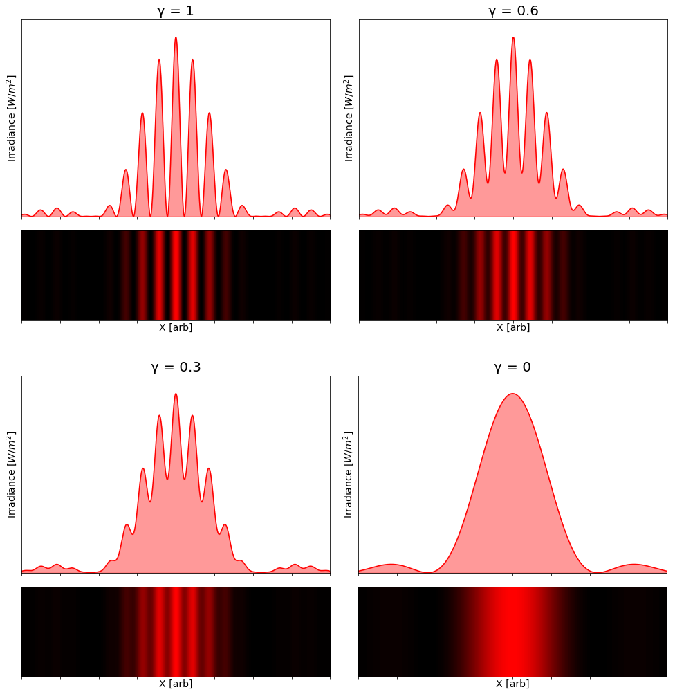
Although \eqref{eq:2} doesn't produce exact results for the scale of these simulations, you can use it for qualitative predictions. When $\left| \gamma \right| = 1$ the fringes are perfectly visible, and when $\left| \gamma \right| = 0$ they cannot be seen. The further you place the light source from the double slit, the closer the coherence degree will be of $1$ .
To illustrate the equation \eqref{eq:2} we have plotted it for different degrees of coherence:
This experiment is important because it's usually the easiest to set up to measure the degree of coherence of a light source. For an experimental discussion see for example [8]. I hope these simulations have helped you to visualize how it really works.
Bibliography
[1] Goodman J W Statistical Optics sec. 5.1 'Spatial Coherence'
[2] Goodman J W Statistical Optics sec. 5.4 'Propagation of the mutual coherence'
[3] Goodman J W Statistical Optics sec. 5.6 'The Van Cittert-Zernike theorem'
[4] M.J. Beran and G.B. Parrent, Jr. Theory of Partial Coherence. Prentice-Hall, Inc., Englewood Cliffs, NJ, 1964.
[5] A.S. Marathay. Elements of Optical Coherence Theory. John Wiley & Sons, New York,NY, 1982.
[6] P.H. van Cittert (1934). "Die Wahrscheinliche Schwingungsverteilung in Einer von Einer Lichtquelle Direkt Oder Mittels Einer Linse Beleuchteten Ebene". Physica. 1 (1–6): 201–210.
[7] F. Zernike (1938). "The concept of degree of coherence and its application to optical problems". Physica. 5 (8): 785–795
[8] Brett J. Pearson, Natalie Ferris, Ruthie Strauss, Hongyi Li, and David P. Jackson, "Measurements of slit-width effects in Young’s double-slit experiment for a partially-coherent source," OSA Continuum 1, 755-763 (2018)