Simulating Light Diffraction with Lenses - Visualizing Fourier Optics
Most interesting and practical optical instruments use lenses to manipulate the formation of images, so understanding how lenses affect the propagation of light is critical to understand Fourier optics.
In the above video, we'll illustrate some of the principles of Fourier optics visually and intuitively by showing how lenses affect the diffraction of light through seven simulations.
In these simulations we'll compare the diffraction patterns with lenses and without it, experiment with different apertures and locations of the lenses while discussing some of their applications.
The simulations were done with the angular spectrum method, which was explained in this post. It's recommended to read this post before entering on this one.
In this post, we'll assume that the reader already knows the fundamentals of geometric optics and diffraction, and we'll discuss deeper the math involved and the optical imaging system simulation (2:03), which also illustrates the diffraction limited systems, that are quite important in microscopy.
Finally, we'll explain how to simulate diffraction patterns using lenses with Python.
Modeling a thin lens as a phase transformation
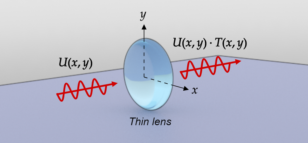
Figure 1: Diagram illustrating a thin lens acting as a phase transformation over the input field
In this section, we'll show how to mathematically modeling a thin lens.
Suppose that a monochromatic wave is incident on a thin lens, On $z = 0$, let the complex field of the wave be represented as:
\begin{equation} u(x, y, 0; t) = U(x, y, 0) e^{-i \omega t} \end{equation}
The lens is said to be a thin lens if a ray that enters at coordinates $(x, y)$ on one face of the lens approximately go out from the other face with a negligible transversal deviation. Then the total phase delay suffered by the wave at coordinates $(x, y)$ in passing through the lens can be written as:
\begin{equation} \phi(x, y)= \frac{2\pi}{\lambda} n \Delta(x, y)+ \frac{2\pi}{\lambda}\left[\Delta_{0}-\Delta(x, y)\right] \end{equation}
where:
$$ \Delta_{0} = \text{maximum thickness of the lens}$$ $$ \Delta (x, y) = \text{thickness at coordinates } (x, y)$$ $$ \lambda = \text{wavelength}$$ $$ n = \text{refractive index of the lens}$$
The term $\frac{2\pi}{\lambda} n \Delta(x, y)$ represents the phase delay introduced by the lens, while $\frac{2\pi}{\lambda}\left[\Delta_{0}-\Delta(x, y)\right]$ is the phase delay introduced by the remaining region of free space between the two planes. Applying this phase delay on a plane immediately in front of the lens leads to:
\begin{equation} U_{l}^{\prime}(x, y) = T(x, y)\cdot U(x, y) \label{eq:3} \end{equation}
where:
\begin{equation} T(x, y) = e^{i \phi(x, y)} \end{equation}
$\phi(x, y)$ is a function of $\Delta (x, y)$ which depends on the geometry of the lens. For a spherical lens with a focal distance equal to $f$ it can be shown that:
\begin{equation} T(x, y)= e^{-i \frac{k}{2 f}\left(x^{2}+y^{2}\right)} \label{eq:5} \end{equation}
The paraxial approximation was used in the above expression. See [1] for a complete proof of this formula.
Equation \eqref{eq:5} and \eqref{eq:3} is all what we need to model a spherical thin lens. After applying the phase delay to the input field $U(x, y)$ we can propagate the output field $U_{l}^{\prime}(x, y)$ using the angular spectrum method.
Simulation of an Optical Imaging System
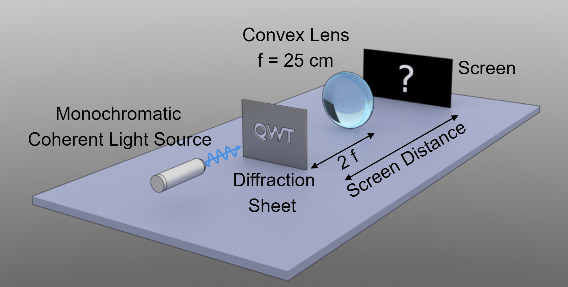
Figure 2: Diagram illustrating the simulation setup of a coherent optical imaging system. This simulation is shown at 2:03.
Probably this is one of the most interesting systems to study when using lenses. This simulation shows the Fourier transforming properties of lenses, their image formation, and the image diffraction limit.
Let first take a look at the system from a geometrical perspective. The distance from the object (here, the QWT aperture) and the lens is $- 2 f$. Then, using the thin lens equation, we find that a real, inverted image is formed at a distance $2 f$ from the lens.
\begin{equation} \frac{1}{2 f} + \frac{1}{2 f} = \frac{1}{f} \end{equation}
Geometrical optics also says that when the screen is placed on the focal point of the lens, it should display a single point, where the thin lens is converging all the incident parallel rays.
Let's check now what happens when we account for diffraction:
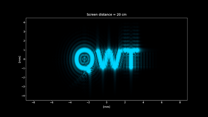
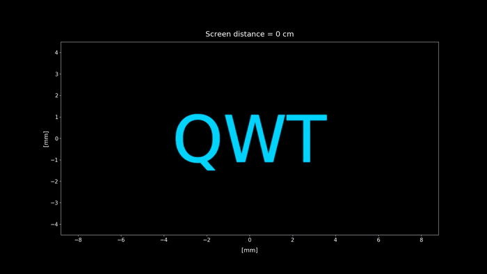
Figure 3: Simulation of the setup shown in figure 2. We change the screen distance from 0 to 100 cm, showing each position diffraction pattern projected on the screen. Click on the play button to display the animation.
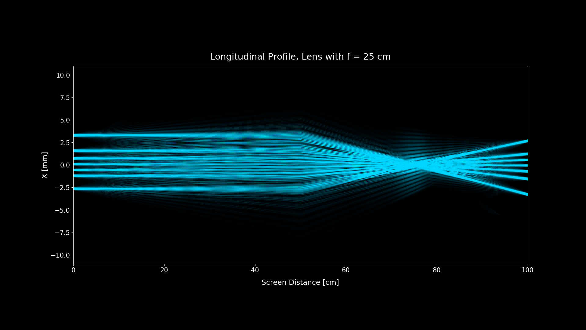
Figure 4: Longitudinal profile (ZX plane slice at y = 0)
When accounting for diffraction, we can see that the pattern on the focal point (screen distance = 75 cm) isn't a single point, as geometrical optics predicts. What the screen is actually showing is the Fourier transform of the aperture.
It just happens that for a typical macroscopic setting, the Fourier pattern shown is too small that it cannot be seen to the naked eye, and it looks like a single point. But when we zoom in to that point, or we decrease the aperture size to increase to the size of the diffracted field, that point starts to exhibit a structure, and that structure is the Fourier transform of the aperture.
For a lens placed a distance $d$ from the aperture when using the Fresnel approximation, it can be shown [2] that the following expression gives the diffracted field on the focal point:
\begin{equation} U^{\prime}(x, y)= \frac{U_0 e^ \left[i \frac{\pi}{f \lambda}\left(1-\frac{d}{f}\right)\left(x^{2}+y^{2}\right)\right]}{i \lambda f} \iint_{-\infty}^{\infty} t_{A}(x^{\prime}, y^{\prime}) e^ \left[-i \frac{2 \pi}{\lambda f}(x^{\prime} x + y^{\prime} y)\right] d x^{\prime} d y^{\prime} \end{equation}
where $t_{A}(x^{\prime}, y^{\prime})$ is the amplitude transmittance function of the aperture.
There is a small detail to highlight: the above expression shows that the diffracted field isn't exactly the Fourier Transform of the aperture because it's multiplied by a phase transformation (except when $d = f$ that vanishes). But when plotting the intensity, which is $I ∝ |U^{\prime}(x, y)|^2$ the phase transformation doesn't make any difference, so we can safely say that the intensity of the diffraction pattern is exactly the squared modulus of the Fourier transform of the aperture.
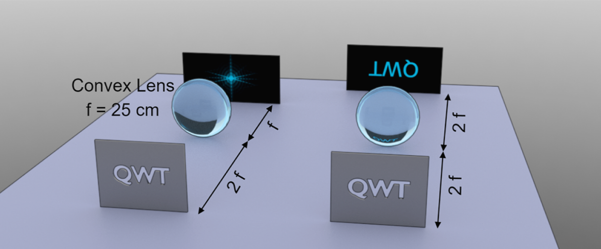
Figure 5: Diffraction patterns when the screen is placed in the focal plane of the lens (left) and the image plane (right)
When the screen is placed at a distance of $2f = 50 \text{ cm}$ from the lens, the diffraction pattern yields an inverted image of the aperture, so at first glance, the geometrical optics result seems correct when accounting diffraction. In the next section, we´ll see that this fact isn't kept true when the size of the aperture is reduced.
The Abbe Diffraction Limit
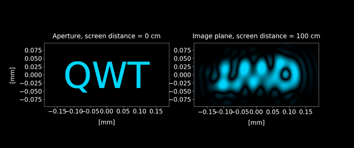
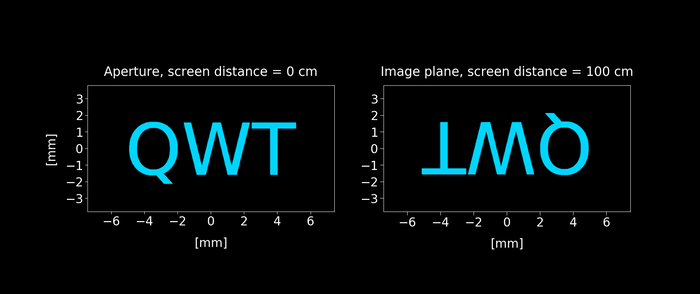
Figure 6: Keeping the setup shown in figure 2 with the screen is placed in the image plane (100 cm from the aperture), we reduce the size aperture from 8mm to 0.2 mm. As the aperture keeps reducing, a wave distortion appears on the image. Click on the play button to display the animation.
In the figure 6, we can see the effect of diffraction on image formation. Let's explain this phenomenon.
Consider first the nature of the image predicted by geometrical optics. If the imaging system is perfect, then the image is inverted and magnified (or demagnified) by a factor $M = -\frac{z_{2}}{z_{1}}$, where $z_{2}$ is the distance from the image to the lens and $z_{1}$ from the lens to the aperture. Thus according to geometrical optics, the image $U_{i}(x, y)$ and the aperture $U_{o}(x, y)$ would be related by:
\begin{equation} U_{i}(x, y)=\frac{1}{|M|} U_{o}\left(\frac{x}{M}, \frac{y}{M}\right) \end{equation}
When we account for the effect of diffraction, the relation can be expressed using a convolution [3] as follows:
\begin{equation} U_{i}(x, y)= h(x, y) \otimes \frac{1}{|M|} U_{o}\left(\frac{x}{M}, \frac{y}{M}\right) =\iint_{-\infty}^{\infty} h(x-x^{'}, y-y^{'})\left[\frac{1}{|M|} U_{o}\left(\frac{x^{'}}{M}, \frac{y^{'}}{M}\right)\right] d x^{'} d y^{'} \label{eq:9} \end{equation}
The function $h(x, y)$ is called amplitude point-spread function and can be expressed as the Fourier transform of the lens pupil:
\begin{equation} h(x, y)= \mathcal{F} \left[ P\left(\lambda z_{2} x^{'}, \lambda z_{2} y^{'}\right) \right] = \iint_{-\infty}^{\infty} P\left(\lambda z_{2} x^{'}, \lambda z_{2} y^{'}\right) e^{-i 2 \pi(x x^{'}+y y^{'})} d x^{'} d y^{'} \label{eq:10} \end{equation}
The lens pupil function $P(x,y)$ represents the finite extension associated with the lens. For a circular lens with radius $R_0$ (used in the simulation shown in figure 6), it is defined as follows:
\begin{equation} P(x, y)=\left\{\begin{array}{ll} 1 & \text{if } r = \sqrt{ x^{2} + y^{2}} < R_0\\ 0 & \text { otherwise } \end{array}\right. \end{equation}
What all of these formulas mean can be better illustrated in the Fourier space. Using the convolution theorem we can express \eqref{eq:9} as a product of the Fourier transform of $h(x, y)$ and $\frac{1}{|M|} U_{o}\left(\frac{x}{M}, \frac{y}{M}\right)$:
\begin{equation} U_{i}(x, y) = \mathcal{F^{-1}} \left[H(f_x, f_y) A_{o}(f_x, f_y)\right] \label{eq:12} \end{equation}
where:
$$H(f_x, f_y) = \mathcal{F} \left[h(x, y)\right] = P\left(-\lambda z_{2} f_x, -\lambda z_{2} f_y\right)$$ $$A_{o}(f_x, f_y) = \mathcal{F} \left[\frac{1}{|M|} U_{o}\left(\frac{x}{M}, \frac{y}{M}\right)\right]$$
$H(f_x, f_y)$ is called Amplitude Transfer Function (ATF) and we see it's only dependent on the pupil lens function.
The expression \eqref{eq:12} supplies very revealing information because it shows that the lens pupil is acting as a low pass filter, removing any spatial frequency of the image higher than:
\begin{equation} f_{coherent} = \frac{r}{λ z_2 } \end{equation}
This fact implies that any detail of the image smaller than $d_{coherent} = \frac{λ z_2}{r}$ is distorted, explaining why the wave distortion shown in Figure 6 appears.
So far, we have used coherent light, but when dealing with spatially incoherent light, we can also express the relation between the images as a convolution, but this time, we use the field intensity instead of the field amplitude, related by:
\begin{equation} I_{i}(x, y)\propto |h(x, y)|^{2} \otimes I_{0}\left(\frac{x}{M}, \frac{y}{M}\right) \end{equation}
And similarly, as we did with the coherent case, we can express this relation in the Fourier space:
\begin{equation} I_{i}(x, y) \propto \mathcal{F^{-1}} \left[\mathcal{H}(f_x, f_y) G_{o}(f_x, f_y)\right] \end{equation}
where:
$$\mathcal{H}(f_x, f_y) = \mathcal{F} \left[|h(x, y)|^{2}\right]$$ $$G_{o}(f_x, f_y) = \mathcal{F} \left[I_{0}\left(\frac{x}{M}, \frac{y}{M}\right)\right]$$
$\mathcal{H}(f_x, f_y)$ is called Optical Transfer Function (OTF) and like the Amplitude Transfer Function (ATF), it's only dependent on the pupil lens function. Furthermore, it can be shown the OTF is the autocorrelation function of the ATF [4].
This implies again the pupil again acts as a low pass filter, but in contrast to coherent imaging, which is linear with the field, incoherent imaging is linear with irradiance, and the cutoff frequency is multiplied by 2:
\begin{equation} f_{incoherent} = 2 f_{coherent} = \frac{2 r}{λ z_2 } \end{equation}
By inverting the above equation, we get the expression for the diffraction-limited spatial resolution $d_{incoherent}$, denominated Abbe diffraction limit [5]:
\begin{equation} d_{incoherent} = \frac{λ}{2 sin(θ)} = \frac{λ}{2 {NA}} \label{eq:Abbe} \end{equation}
We have defined $θ$ is the half-angle to which the optical system is focusing the light. Note that because we are using the paraxial approximation we can set $tan θ = \frac{z_2}{r} \approx sin θ$. However, $sin θ$ is preferred because it illustrates that the maximum resolution achievable is never going to be smaller than the wavelength $λ$.
The term ${NA} =\sin \theta$ is called numerical aperture and it's commonly used in microscopy. When the medium in which the lens has a index of refraction $n$, we can further generalize \eqref{eq:Abbe} by dividing it by $n$. In this case, the numerical aperture is defined as ${NA} =n \sin \theta$:
A lens with a larger numerical aperture will be able to visualize finer details than a lens with a smaller numerical aperture, thus making useful using a medium with a high index of refraction.
Note that the Abbe diffraction limit is not absolute. Resolution beyond this diffraction limit can be achieved in some special cases, by using, for example, evanescent fields or strong non-linear effects [6].
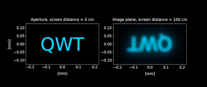
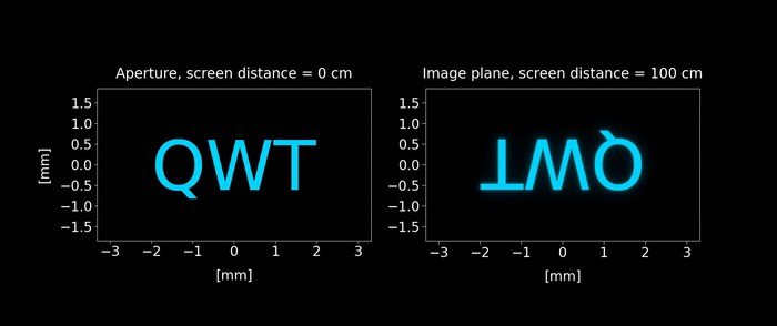
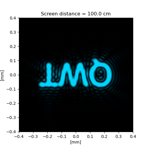
Figure 7: Simulated diffraction-limited spatially incoherent image. Unlike the coherent case shown in figure 6, the wave interferences are less visible and the image diffraction limit distorsion is mostly due a blurring effect.
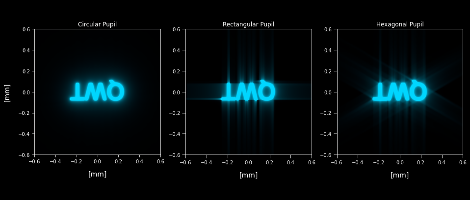
Figure 8: Simulated diffraction-limited spatially incoherent image for different pupil shapes.
The simulations shown in Figures 6 and 7 use circular-shaped pupils, but when pupils with hard edges are used, diffraction spikes are visible in the image. This phenomenon can be seen in normal vision, due to the diffraction through eyelashes and the edges of the eyelids when one is squinting staring a light. In the case of photography, the diffraction spikes are due the iris diaphragms of camera lenses.
Implementation with Python
The simulations of the video can be found on the GitHub repository. In this section, we are going to show the implementation of the two simulations discussed.
The simulation shown in the figure 3 can be reproduced with the following script. The example uses the module diffractsim discussed in the angular spectrum method post. It's necessary to place the image acting as the QWT aperture on the path "./apertures/QWT.jpg" respective to the folder where the script is executed.
import diffractsim
diffractsim.set_backend("CUDA") #Change the string to "CUDA" to use GPU acceleration

from diffractsim import MonochromaticField, ApertureFromImage, Lens, nm, mm, cm, um


zi = 50*cm # distance from the image plane to the lens
z0 = 50*cm # distance from the lens to the current position
M = zi/z0 # magnification factor
radius = 6*mm
NA = radius  / z0  #numerical aperture

#print diffraction limit
print('\n Maximum object resolvable distance by Rayleigh criteria: {} mm'.format("%.3f"  % (0.61*488*nm/NA /mm)))


# set up simulation
F = MonochromaticField(
    wavelength=488 * nm, extent_x=1.5 * mm, extent_y=1.5 * mm, Nx=2048, Ny=2048,intensity = 0.2
)

F.add(ApertureFromImage("./apertures/QWT.png",  image_size = (1.0 * mm, 1.0 * mm), simulation = F))

F.scale_propagate(z0, scale_factor = 30)
#zi and z0 must satisfy the thin les equation 1/zi + 1/z0 = 1/f
F.add(Lens(f = zi*z0/(zi+z0), radius = radius))
F.scale_propagate(zi, scale_factor = M/(30))

#image at z = 100*cm
rgb = F.get_colors()
F.plot_colors(rgb, figsize=(5, 5), xlim=[-0.5*mm,0.5*mm], ylim=[-0.5*mm,0.5*mm])
The above script can also reproduce the simulation shown in figure 6, however, in order to correctly simulate the optical system we need two propagations.
This computation can be simplified by performing the convolution \eqref{eq:9} through succesive Fourier transforms, applying the convolution theorem as revealed in \eqref{eq:10}. This approach avoid computing the field at lens position, that due the big extent of the diffracted field at the lens, requires reescaling the diffraction plane, at least, by a factor of 30.
The following script is presented with this fast approach to reproducing the results of figure 6.
import diffractsim
diffractsim.set_backend("CPU")
from diffractsim import MonochromaticField,ApertureFromImage, nm, mm, cm,um, CircularAperture

zi = 50*cm # distance from the image plane to the lens
z0 = 50*cm # distance from the lens to the current position
M = -zi/z0 # magnification factor
radius = 6*mm
NA = radius  / z0  #numerical aperture

#print diffraction limit
print('\n Maximum object resolvable distance by Rayleigh criteria: {} mm'.format("%.3f"  % (0.61*488*nm/NA /mm)))


F = MonochromaticField(
    wavelength=488 * nm, extent_x=1.5 * mm, extent_y=1.5 * mm, Nx=2048, Ny=2048,intensity = 0.2
)

F.add(ApertureFromImage("./apertures/QWT.png",  image_size = (1.0 * mm, 1.0 * mm), simulation = F))

F.propagate_to_image_plane(pupil = CircularAperture(radius = 6*mm) , M = M, zi = zi, z0 = z0)
rgb = F.get_colors()
F.plot_colors(rgb, figsize=(5, 5), xlim=[-0.5*mm,0.5*mm], ylim=[-0.5*mm,0.5*mm])
We have defined a function named propagate_to_image_plane that accomplish the computation of \eqref{eq:9} and \eqref{eq:10}. When running the first script, it would yield an inverted image of the QWT aperture, while the second in which a smaller extent_x and extent_y is used, a wave distortion appears. We encourage the reader to change these values and experiment with different magnifications.
optical_imaging_system_using_convolution.pyReferences
[1] Introduction to Fourier Optics J. Goodman sec. 5.1 'A thin lens as a phase transformation'
[2] Introduction to Fourier Optics J. Goodman sec. 5.2 'Fourier transforming properties of lenses'
[3] Introduction to Fourier Optics J. Goodman sec. 5.3 'Image formation: monochromatic illumination'
[4] Introduction to Fourier Optics J. Goodman sec. 6.3 'Frequency response for diffraction-limited incoherent imaging'
[5] Abbe, E. A Contribution to the Theory of the Microscope and the nature of Microscopic Vision. Archiv für Mikroskopische Anatomie 9, 413–418 (1873)
[6] Minin, Igor & Minin, Oleg. (2016). Diffractive Optics and Nanophotonics: Resolution Below the Diffraction Limit.