Simulating Diffraction Patterns with the Angular Spectrum Method and Python

In this project we will show how to numerically compute Diffraction Patterns with the Angular Spectrum Method. We'll implement the method with Python and discuss how to simulate them both with monochromatic and polychromatic light like it's shown in the video above.

The Angular Spectrum

In a previous post we have discussed how to solve the Fresnel Integral with a single Fast Fourier Transform (FFT). However although this method is quite simple, it has some drawbacks:
It is limited by the requirement of a different grid scale than the aperture figure, and by the approximations of the Fresnel and Fraunhofer regimes.
As we will see next, the The Angular Spectrum Method is free of these problems. It uses the same scale that the aperture figure, and it solves the wave equation exactly.

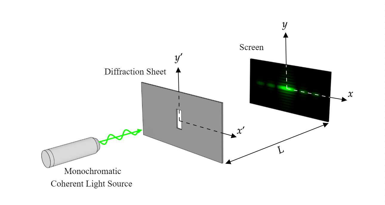
Suppose that a monochromatic wave is incident on a transverse $(x', y')$ plane traveling with a component of propagation in the negative $z$ direction. Let the complex field across that $z = 0$ plane (Diffraction Sheet) be represented by:

$$u(x', y', 0; t) = U(x', y', 0) e^{-\omega t i}$$

Our ultimate objective is to calculate the resulting field $U(x, y, -L)$ that appears across a second, parallel plane (Screen) a distance $L$ to the right of the first plane.

Across the $z = 0$ plane, the function $U(x, y, 0)$ has a two-dimensional Fourier transform given by:

\begin{equation} A\left(k_{x}, k_{y} ; 0\right)=\int_{-\infty}^{\infty} \int_{-\infty}^{\infty} U(x', y', 0) e^{-(k_{x} x' + k_{y} y') i} \mathrm{d} x' \mathrm{dy'} \label{eq:1} \end{equation}

where $A\left(k_{x}, k_{y} ; 0\right)$ is called the angular spectrum of the distrubance $U(x, y, 0)$

Propagation of the Angular Spectrum

Consider now the angular spectrum of the disturbance $U(x, y, 0)$ across a plane parallel to the $z = 0$ plane but at a distance z from it. Let the function $A(k_{x}, k_{y}, z)$ represent the angular spectrum of $U(x, y, z)$; that is

\begin{equation} A\left(k_{x}, k_{y} ; z\right)=\int_{-\infty}^{\infty} \int_{-\infty}^{\infty} U(x, y, z) e^{-(k_{x} x + k_{y} y) i} \mathrm{d} x \mathrm{dy} \label{eq:2} \end{equation}

and with its inverse transform given by:

\begin{equation} U\left(x, y , z\right)=\int_{-\infty}^{\infty} \int_{-\infty}^{\infty} A(k_{x}, k_{y}; z) e^{(k_{x} x + k_{y} y) i} \mathrm{d} k_{x} \mathrm{d} k_{y} \label{eq:3} \end{equation}

To know how the disturbance $U(x, y, z)$ varies with $z$, we are going to use the Helmholtz equation \eqref{eq:4} which is obtained simply from the wave equation after separating the temporal part:

\begin{equation} \nabla^{2} U + k^{2} U=0 \quad \text{with} \quad k = \frac{2 \pi}{\lambda} \label{eq:4} \end{equation}

Now if we plug equation \eqref{eq:3} into the Helmholtz equation we obtain the following relationship:

\begin{equation} \frac{d^{2}}{d z^{2}} A + k_{z} A = 0 \quad \text{with} \quad k_{z} = \sqrt{k^2 - k_{x}^2 + k_{y}^2} \label{eq:5} \end{equation}

which has the solution:

\begin{equation} A{\left(k_{x},k_{y}; z \right)} = A{\left(k_{x},k_{y}; 0 \right)} e^{- k_{z} z i} \label{eq:6} \end{equation}

Finally, we note that the disturbance observed at $z = -L$ can be written in terms of the initial angular spectrum by inverse transforming \eqref{eq:6} using \eqref{eq:3}, giving:

\begin{equation} U\left(x, y , -L\right)=\int_{-\infty}^{\infty} \int_{-\infty}^{\infty} A(k_{x}, k_{y}; 0) e^{k_{z} L} e^{(k_{x} x + k_{y} y) i} \mathrm{d} k_{x} \mathrm{d} k_{y} \label{eq:7} \end{equation}

Now, we define the amplitude transmittance function $t_{A}(x', y')$ of the aperture as the ratio of the transmitted field amplitude $U(x', y', 0)$ to the incident field amplitude $U_{0}(x, y, 0)$ at each $(x, y)$ in the $z = 0$ plane:

\begin{equation} U(x', y', 0)=U_{0}(x', y', 0) t_{A}(x', y') \label{eq:8} \end{equation}

The amplitude transmittance function has the value 1 at $(x, y)$ if light can pass through it, and 0 if it cannot. So it represents the shape of the aperture.

The equations \eqref{eq:8}, \eqref{eq:1} and \eqref{eq:7} are everything we need to compute the electric field at $z = -L$. In order to accomplish such task, we realize that realize that \eqref{eq:1} and \eqref{eq:7} can be represented as Fast Fourier Transforms (FFT) as follows:

First, we discretize the region $(x', y') \in [-L_{x},L_{x}] \times [-L_{y},L_{y}]$ dividing each axis in $N_{x}$ and $N_{y}$ points respectively:

$$ \begin{gathered} x_{s_{x}}^{\prime}= \left\{ -L_{x}+s_{x} \frac{2 L_{x}}{N_{x}}: 0 \leq s_{x} \leq N_{x}-1 \right\} \\ y_{s_{y}}^{\prime}= \left\{ -L_{y}+s_{y} \frac{2 L_{y}}{N_{y}}: 0 \leq s_{y} \leq N_{y}-1 \right\} \end{gathered} $$

Now we express \eqref{eq:1} as the Discrete Fourier Transform (DFT) of that set of points, which we will efficiently compute using the Fast Fourier Transform (FFT) algorithm:

\begin{equation} c\left(n_x,n_y\right)=\sum_{s_x=0}^{N_x-1}\sum_{s_y=0}^{N_y-1}{U\left(x_{s_x}^{\prime},\ y_{s_y}^{\prime}, 0\right)e^{i\frac{-2\pi s_x}{N_x}n_x}e^{i\frac{-2\pi s_y}{N_y}n_y}} \label{eq:9} \end{equation}

And \eqref{eq:7} with the inverse Fast Fourier Transform (iFFT):

\begin{equation} U\left(x_{s_x},y_{s_y},-\ L\right)=\frac{1}{N_xN_y}\sum_{n_x=\frac{N_x}{2}}^{\frac{N_x}{2}-1}\sum_{n_y=-\frac{N_y}{2}}^{\frac{N_y}{2}-1}{c\left(n_x,n_y\right)e^{ik_zL}e^{i\frac{2\pi n_y}{N_x}s_x}e^{i\frac{2\pi n_y}{N_y}s_y}} \label{eq:10} \end{equation}

where:

$$ k_z = \sqrt{ \left( \frac{2 \pi}{\lambda} \right)^{2} - \left(\frac{\pi n_{x}}{L_{x}} \right)^{2} - \left(\frac{\pi n_{y}}{L_{y}} \right)^{2} } $$

Finally, we get the intensity of the diffraction pattern in the screen plane by multiplying $U$ by its conjugate:

\begin{equation} I\left(x,y,-L\right) \propto{\ U}^\ast\left(x,y,-L\right) \cdot U\left(x,y,-L\right) \label{eq:11} \end{equation}

In the Implementation with Python section will translate \eqref{eq:8}, \eqref{eq:9}, \eqref{eq:10} and \eqref{eq:11} in to computer code using Python scientific packages numpy and scipy.

Implementation with Python

All of the source code of the implementation can be found in its GitHub repository. In this section we are going to show a brief description of it.

We have defined and created a class named MonochromaticField that will serve as the simulation interface. This class is initialized with the arguments wavelength, extent_x, extent_y, Nx, Ny. extent_x, extent_y are the length and height of the rectangular grid and Nx, Ny the dimension of the grid respectively.

The class MonochromaticField contains a method called add(ApertureFromImage(amplitude_mask_path, image_size, simulation)) This method load an image specified as a string with the argument amplitude_mask_path . The image is supposed to be a greymap and will serve as the amplitude transmittance function $t_{A}(x', y')$ defined in \eqref{eq:8}. White pixels will be loaded as value 1 and black pixels as 0.
The image is centered on the plane and its physical size is specified in image_size argument as image_size = (float, float) If image_size isn't specified, the image fills the entire aperture plane.

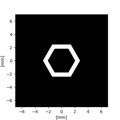
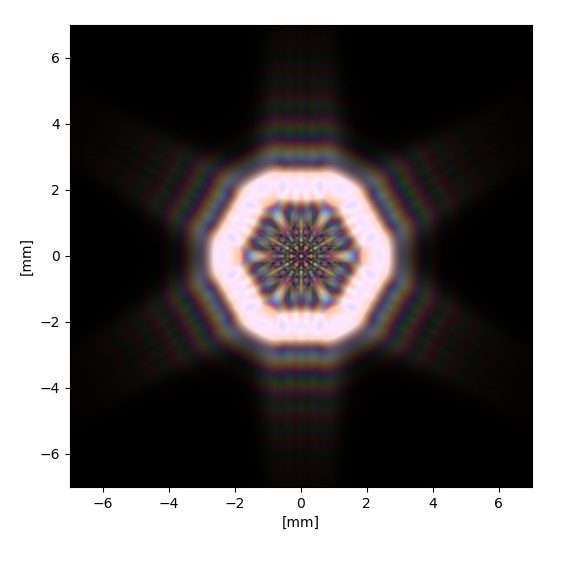
The image below is an image of an outline hexagon aperture loaded with ApertureFromImage class:

Finally, we can compute the diffraction pattern at a specified distance z with compute_colors_at(z).
This method will compute \eqref{eq:9}, \eqref{eq:10} and \eqref{eq:11} making use of the FFT algorithm implemented with scipy.
The method return an array of RGB colors with the same dimension of the aperture, that later can be plotted with plot(self,rgb, figsize=(6,6), xlim = None, ylim = None) making use of the matplotlib library.

As an example of the methods explained, we present here the source code to simulate the diffraction pattern of the above outline hexagon:

import diffractsim
diffractsim.set_backend("CPU") #Change the string to "CUDA" to use GPU acceleration

from diffractsim import MonochromaticField, ApertureFromImage, mm, nm, cm

F = MonochromaticField(
    wavelength=632.8 * nm, extent_x=18 * mm, extent_y=18 * mm, Nx=1024, Ny=1024
)

F.add(ApertureFromImage("./apertures/hexagon.jpg", image_size=(5.6 * mm, 5.6 * mm), simulation = F))


F.propagate(80*cm)
rgb = F.get_colors()
F.plot_colors(rgb, xlim=[-7* mm, 7* mm], ylim=[-7* mm, 7* mm])

When this script is run with different wavelengths, it will return the following diffraction patterns:

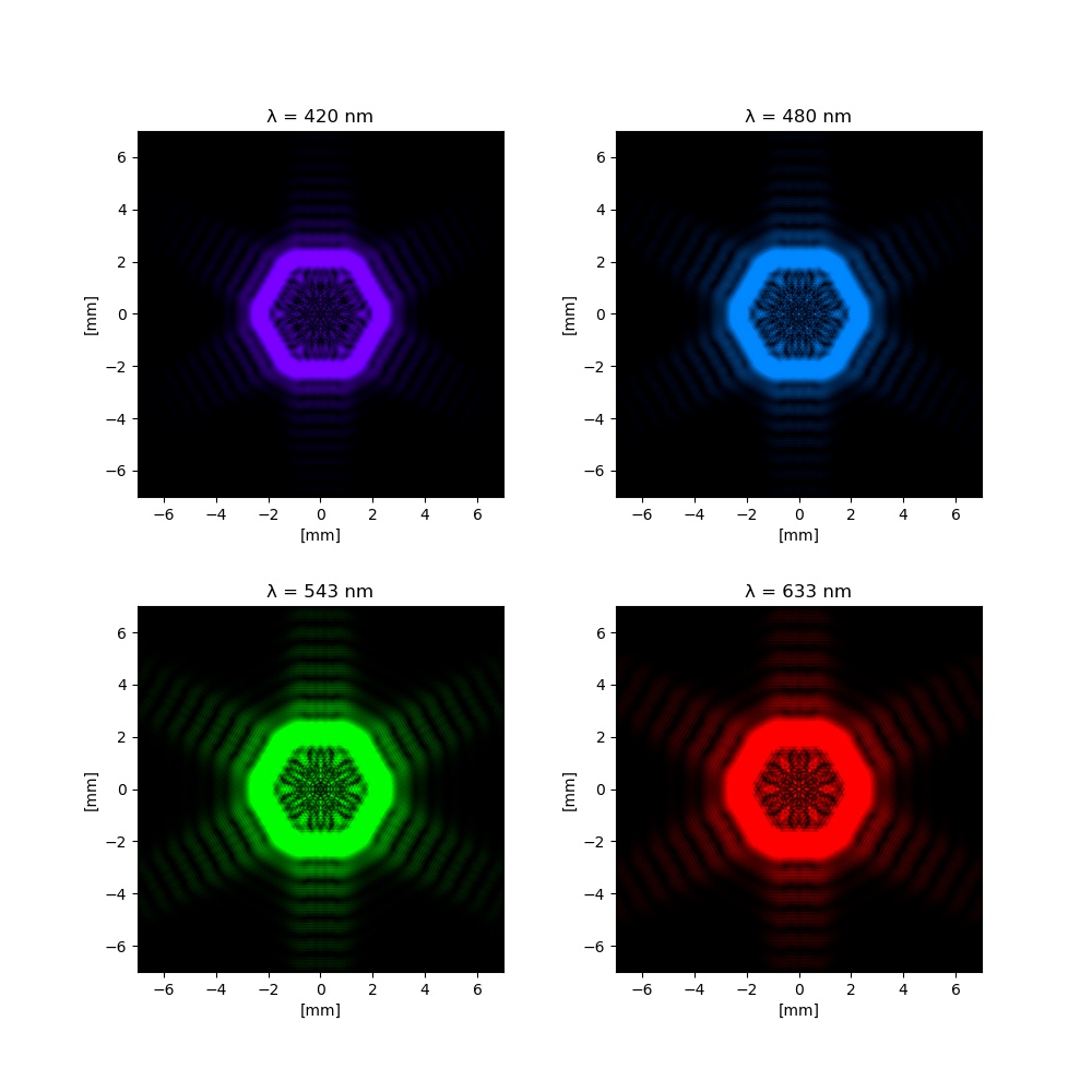
As we can see in the plots, the higher the light's wavelength, the longer the diffraction pattern is. Note as well that the green diffraction pattern is the brightest. That is because the human eye presents peak sensitivity at about 555 nanometers.

Polychromatic Light

For getting the total field that irradiates on the screen for a broad spectrum, we must compute $U(x, y, -L)$ for each wavelength and integrate it over the entire spectrum. But what we are going to show here is how to compute the colors produced by the diffraction pattern in a way that can be displayed by a computer monitor. This can be achieved using CIE's color matching functions.
These are three integrals $\hat{x}(\lambda), \hat{y}(\lambda) \text { and } \hat{z}(\lambda)$ that describe the chromatic response of the observer as a function of the wavelength yielding to CIE tristimulus values $X, Y \text { and } Z$:

\begin{equation} \begin{aligned} X &=\int_{\lambda} L(\lambda, x, y) \hat{x}(\lambda) d \lambda \\ Y &=\int_{\lambda} L(\lambda, x, y) \hat{y}(\lambda) d \lambda \\ Z &=\int_{\lambda} L(\lambda, x, y) \hat{z}(\lambda) d \lambda \end{aligned} \label{eq:12} \end{equation}

$L(\lambda, x, y)$ is defined as the spectral radiance reflected on the screen at the point $(x,y)$. We will consider that the screen is a diffuse surface, and its reflectance is given by the Lambert law. As a consequence, the relation of the incident intensity and the reflected radiance can be expressed as:

\begin{equation} L(\lambda, x, y) = \frac{R}{\pi} \cdot I(\lambda, x,y) \label{eq:13} \end{equation}

where:

$$I(\lambda, x,y) = \text{ Spectral irradiance on the screen at the point (x,y)}$$ $$R = \text{ Reflectance of the diffuse surface}$$

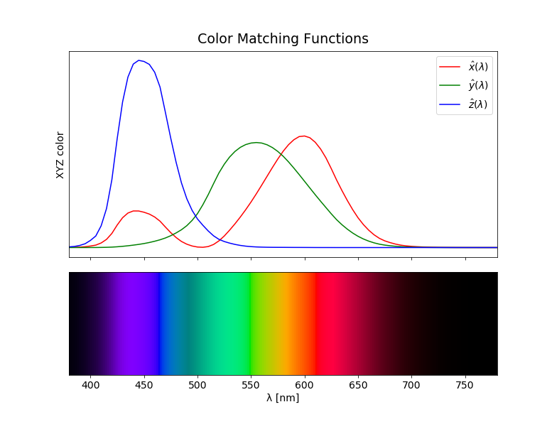
The tabulated values of the CIE's color matching functions can be found in cie-cmf.txt. The $X, Y \text { and } Z$ values can be transformed to some RGB space to be displayed. For example, assuming standard sRGB primaries and white point we have the following relation for the RGB values:

$$ \left[\begin{matrix}R\\G\\B\end{matrix}\right] = \left[\begin{matrix}3.2406 & -1.5372 & -0.4986\\-0.9689 & 1.8758 & 0.0415\\0.0557 & -0.204 & 1.057\end{matrix}\right] \left[\begin{matrix}X\\Y\\Z\end{matrix}\right] $$

There is one step more to do. The human eye doesn't perceive the color intensity linearly, so this is the reason that we apply a gamma correction to the final RGB values:

$$ RGB_{out} = \begin{cases} 12.92 \cdot RGB_{linear} & \text{for}\: RGB_{linear} \leq 0.00304 \\1.055 \cdot RGB_{linear}^{0.42} - 0.055 & \text{otherwise} \end{cases} $$

All of the transformations described has been implemented in colour_functions.py:

For computing diffraction patterns for broad spectrums, we have defined the class PolychromaticField which has an analogous role to MonochromaticField defined before.

This class is initialized with the arguments spectrum, extent_x, extent_y, Nx, Ny.

spectrum must be an array with spectral intensity if light sampled on 380-780 nm interval, while the last four arguments are the same ones defined for MonochromaticField

The method compute_colors_at now has two new arguments: spectrum_size is the number of samples of the spectrum.
spectrum_divisions is the number of divisions of the spectrum that will be used for computing the integrals \eqref{eq:12}. A higher value will return to more accurate colors.
An important note: spectrum_size/spectrum_divisions should be an integer.

The complete implementation of this class can be found in polychromatic_simulator.py

Now we are going to give an example of how to use this class. We are going to use the outline hexagon aperture from the previous example, but this time using a white light spectrum. This can be achieved using the Illuminant D65 whose sample list can be found in illuminant_d65.txt.

import diffractsim
diffractsim.set_backend("CPU") #Change the string to "CUDA" to use GPU acceleration

from diffractsim import PolychromaticField, ApertureFromImage, cf, mm, cm

F = PolychromaticField(
    spectrum=2 * cf.illuminant_d65, extent_x=18 * mm, extent_y=18 * mm, Nx=1024, Ny=1024
)

F.add(ApertureFromImage("./apertures/hexagon.jpg", image_size=(5.6 * mm, 5.6 * mm), simulation = F))

F.propagate(z=80*cm)

rgb =F.get_colors()
F.plot_colors(rgb, xlim=[-7* mm, 7* mm], ylim=[-7* mm, 7* mm])

This script returns the following plot:

Final discussion

The source code uploaded allows simulating arbitrary diffraction patterns with only 8 lines of code, making its possible study easier.

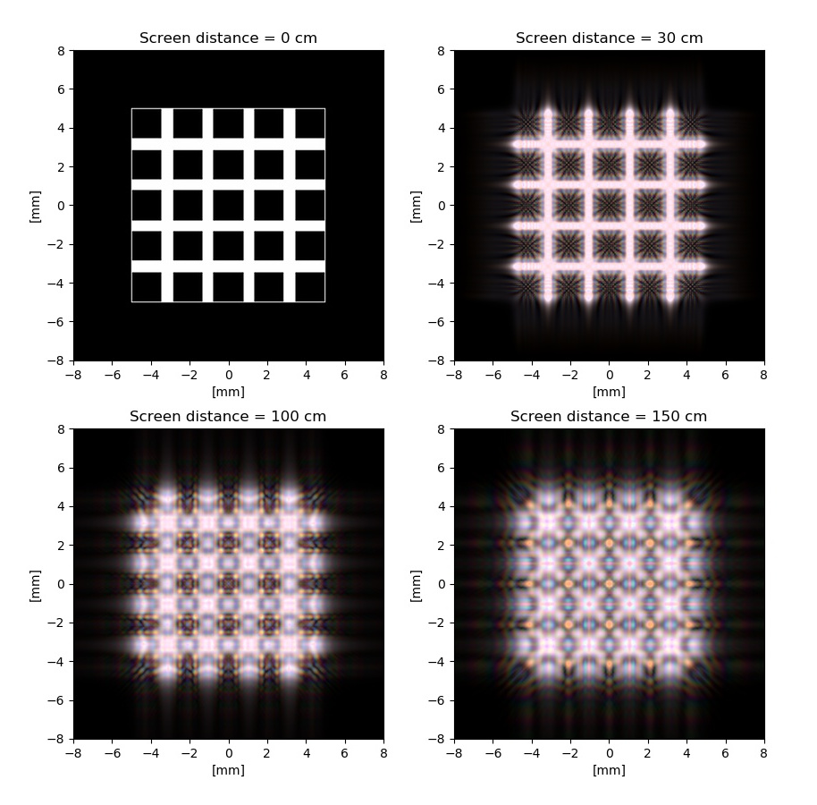
A remarkable characteristic observed is how much the diffraction patterns change with increasing the screen distance or decreasing the aperture size. For example, let's take a look at the rectangular grating aperture showed in the image below.

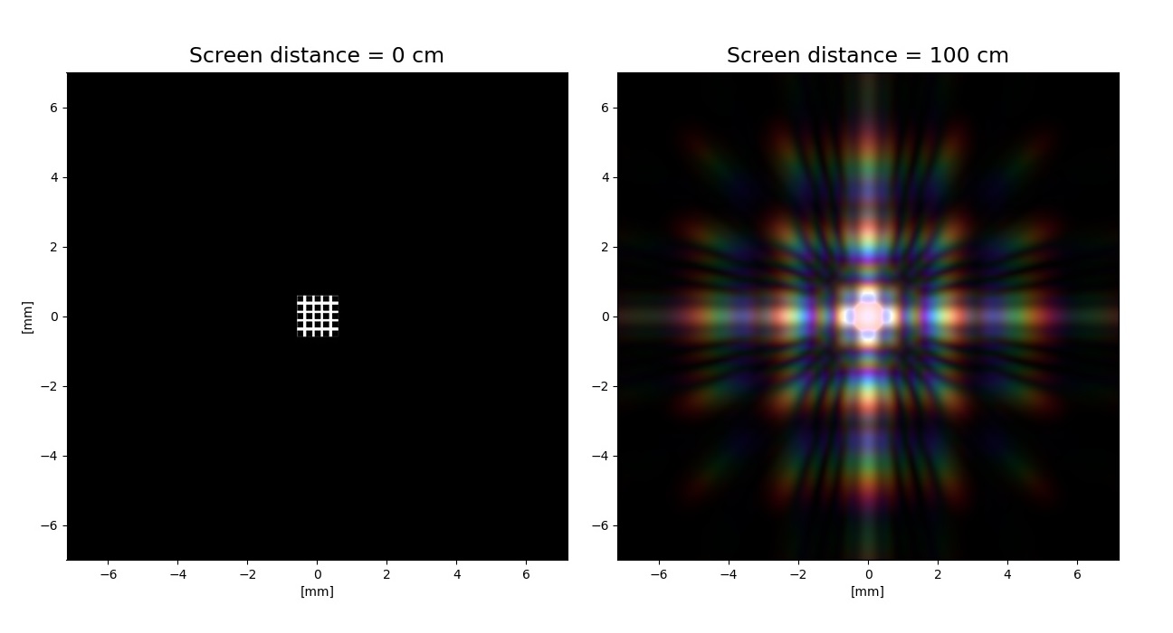
In the next post, we´ll see how to add lenses to our simulations and we'll visualize the principles of Fourier optics:

• Simulating Light Diffraction with Lenses - Visualizing Fourier Optics