Solving the Diffraction Integral with the Fast Fourier Transform (FFT) and Python
In this project we will show how to numerically compute the Fresnel Diffraction Integral with the Fast Fourier Transform (FFT). We'll implement the method with Python and we will apply it to the study of the diffraction patterns produced by the particle beams in the double slit experiment, showing the dependence of the phenomenon with respect to the separation of the slits.
Theoretical model
Consider a particle traveling with a well-defined momentum:
$$ \mathbf {p} = p_ {0} \mathbf {u_ {z}} \quad \text{ in the region }\quad z < 0 $$
Its wave function is:
$$ \Psi{(\mathbf{r},t)} = \Psi_{0} e^{i (k z - w t)},\quad \text{ with } \quad \begin{gathered} \begin{cases} k = \frac{p_{0}}{\hbar} \\ w = \frac{p_{0}^{2}}{2 m \hbar} \\ \end{cases} \end{gathered} $$
A plate is now placed at $ z = 0 $ with an opening $ S '$. According to the Huygen-Fresnel principle which can be derived applying the Rayleigh-Sommerfeld method [1] to the Schrödinger Equation, the wave function in the plane $ z = L $ it's given by the Fresnel integral:
$$ \Psi{(\mathbf{r},t)} = C \int\nolimits_{S'}^{} \frac{e^{i k \left|{r - r'}\right|}}{\left|{r - r'}\right|} cos{\theta}\, d^{2}r', \quad \text{ with } \quad \hspace{2mm} C = \frac{k \Psi_{0} e^{- i t w}}{2 \pi i} $$
This approximation is valid if $ L >> \lambda $
Next we are going to simplify the integral using the Fresnel approximation. This consists of assuming $ \theta \approx 0 $ and using the approximation in the exponential:
$$ |{r - r'}| \approx z +\frac{(x - x')^{2} + (y - y')^{2}}{2 z} $$
Which it is valid if $((x - x')^{2} + (y - y')^{2})^{2} << 8 \lambda L^{3}$
In the case of the denominator, we do:
$$ |{r - r'}| \approx L $$
And the Fresnel integral becomes:
\begin{equation} \begin{gathered} \Psi{(\mathbf{r},t)} = R \int\nolimits_{-\infty}^{\infty}\int\nolimits_{-\infty}^{\infty} f{(x', y')} e^{\frac{i k}{2 z} ({x'}^{2} + {y'}^{2})} e^{ -\frac{i k x}{z}x' -\frac{i k y}{z}y'} \, dx'dy', \hspace{3mm} with \hspace{3mm} R = \frac{k \Psi_{0} e^{ i(k z - t w)}}{2 \pi i z} e^{ i k\frac{x^{2} + y^{2}}{2 z}} \\ f(x', y') = \begin{cases} 1 & \text{ if } (x' , y') \in S' \\ 0 & \text{ if } (x' , y') \notin S'\\ \end{cases} \end{gathered} \end{equation}
Finally, we observe that this integral can be expressed as a Fourier transform:
$$ \begin{gathered} \Psi{(\mathbf{r},t)} =R \hspace{2mm}\mathcal{F} \left[f{(x', y')} e^{\frac{i k}{2 z} ({x'}^{2} + {y'}^{2})} \right] \\ \mathcal{F} \left[f{(x', y')} e^{\frac{i k}{2 z} ({x'}^{2} + {y'}^{2})} \right] = \int\nolimits_{-\infty}^{\infty}\int\nolimits_{-\infty}^{\infty} f{(x', y')} e^{\frac{i k}{2 z} ({x'}^{2} + {y'}^{2})} e^{ -\frac{i k x}{z}x' -\frac{i k y}{z}y'} \, dx'dy' \end{gathered} $$
To estimate the diffraction pattern, we use the region $(x', y') \in [-L_{x},L_{x}] \times [-L_{y},L_{y}]$ dividing each axis in $N_{x}$ and $N_{y}$ points respectively:
$$ \begin{gathered} x_{n_{x}}^{\prime}= \left\{ -L_{x}+n_{x} \frac{2 L_{x}}{N_{x}}: 0 \leq n_{x} \leq N_{x}-1 \right\} \\ y_{n_{y}}^{\prime}= \left\{ -L_{y}+n_{y} \frac{2 L_{y}}{N_{y}}: 0 \leq n_{y} \leq N_{y}-1 \right\} \end{gathered} $$
We define the Discrete Fourier Transform (DFT) of the set of points, which we will efficiently compute using the Fast Fourier Transform (FFT) algorithm:
$$ \begin{gathered} G(\mu_{x}, \mu_{y}) = \sum _{n_{x}=0}^{N_{x}-1}\sum _{n_{y}=0}^{N_{y}-1}g(x'_{n_{x}},y'_{n_{y}})e^{-{i2\pi \mu_{x}{\frac {n_{x}}{N_{x}}} -{i2\pi \mu_{y}{\frac {n_{y}}{N_{y}}}}}}, \end{gathered} $$
With the points of the screen located at $z = L$:
$$ \begin{gathered} x_{\mu_{x}} = \frac{(\mu_{x} - N_{x}/2) L \lambda}{2 L_{x}} \\\\ y_{\mu_{y}} =\frac{(\mu_{y} - N_{y}/2) L \lambda}{2 L_{y}} \end{gathered} $$
And the intensity (probability density) on the screen:
$$ I \propto|G(\mu_{x}, \mu_{y})|^{2} $$
Implementation with Python
To perform the required computations, the following scripts were written in the Python programming language, making use of its scientific packages numpy, scipy and matplotlib.
First we have defined and created a class named Sheet that contains the variables $L_{y} , L_{x}, N_{x}, N_{y}, x_{n_{x}}^{\prime}, y_{n_{y}}^{\prime} $ and an array of points named f, with a value of $1$ in the case that the point of the slit represents a slit $(x_{n_{x}}^{\prime} , y_{n_{y}}^{\prime}) \in S' $ and $0$ otherwise.
import numpy as np

class Sheet():
    def __init__(self,extent_x, extent_y, Nx, Ny):

        self.dx = extent_x/Nx
        self.dy = extent_y/Ny

        self.x = self.dx*(np.arange(Nx)-Nx//2)
        self.y = self.dy*(np.arange(Ny)-Ny//2)
        self.xx, self.yy = np.meshgrid(self.x, self.y)

        self.Nx = int(Nx)
        self.Ny = int(Ny)
        self.E = np.zeros((self.Ny, self.Nx))


    def rectangular_slit(self,x0, y0, lx, ly):
        """
        Creates a slit centered at the point (x0, y0) with width lx and height ly
        """
        self.E += np.select( [((self.xx > (x0 - lx/2) ) & (self.xx < (x0 + lx/2) )) & ((self.yy > (y0 - ly/2) ) & (self.yy < (y0 + ly/2) )),  True], [1, 0])
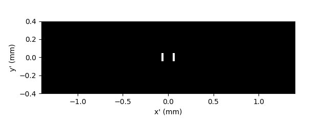
As an example we study the diffraction pattern caused by two rectangular slits separated by a distance D with width and height denoted by lx, ly respectively.
The higher the values of Nx, Ny, Lx, Ly, more accurate the diffraction pattern will be.
Lx = 1.4
Ly = 0.4
Nx= 2500
Ny= 1500

sheet = Sheet(extent_x = 2*Lx , extent_y = 2*Ly, Nx= Nx, Ny= Ny)

#slit separation
mm = 1e-3
D = 128 * mm

sheet.rectangular_slit(x0 = -D/2, y0 = 0, lx = 22 * mm , ly = 88 * mm)
sheet.rectangular_slit(x0 = +D/2, y0 = 0, lx = 22 * mm , ly = 88 * mm)
Next we calculate the Diffraction integral using the Fast Fourier Transform (FFT) algorithm, efficiently implemented with the Scipy function fft2
# distance from slit to the screen (mm)
z = 5000

# wavelength (mm)
λ = 18.5*1e-7
k = 2*np.pi/λ

from scipy.fftpack import fft2
from scipy.fftpack import fftshift

fft_c = fft2(sheet.E * np.exp(1j * k/(2*z) *(sheet.xx**2 + sheet.yy**2)))
c = fftshift(fft_c)
Results: Plotting the diffraction patterns
Finally, we represent the results stored in the numpy array c with matplotlib.
#plot with matplotlib
import matplotlib.pyplot as plt

fig = plt.figure(figsize=(6, 6))
ax1 = fig.add_subplot(2,1,1)
ax2 = fig.add_subplot(2,1,2,sharex=ax1, yticklabels=[])

abs_c = np.absolute(c)

#screen size mm
dx_screen = z*λ/(2*Lx)
dy_screen = z*λ/(2*Ly)
x_screen = dx_screen * (np.arange(Nx)-Nx//2)
y_screen = dy_screen * (np.arange(Ny)-Ny//2)


ax1.imshow(abs_c, extent = [x_screen[0], x_screen[-1]+dx_screen, y_screen[0], y_screen[-1]+dy_screen], cmap ='gray', interpolation = "bilinear", aspect = 'auto')

ax2.plot(x_screen, abs_c[Ny//2]**2, linewidth = 1)

ax1.set_ylabel("y (mm)")
ax2.set_xlabel("x (mm)")
ax2.set_ylabel("Probability Density $|\psi|^{2}$")
ax1.set_xlim([-2,2])
ax2.set_xlim([-2,2])
ax1.set_ylim([-1,1])
plt.setp(ax1.get_xticklabels(), visible=False)


plt.show()
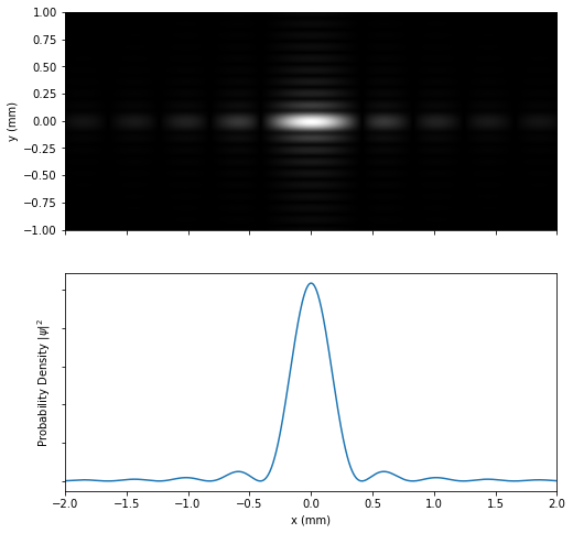
First, We have represented the diffraction pattern of a particle with $\hspace{1mm} λ = 18.5 \text{ Å} \hspace{1mm}$ due to a slit width $\hspace{1mm} 22 × 10^{-3} \text{ mm} \hspace{1mm}$ and height $\hspace{1mm} 88 × 10^{-3} \text{ mm}$, with the screen placed at $5 \text{ m}$:
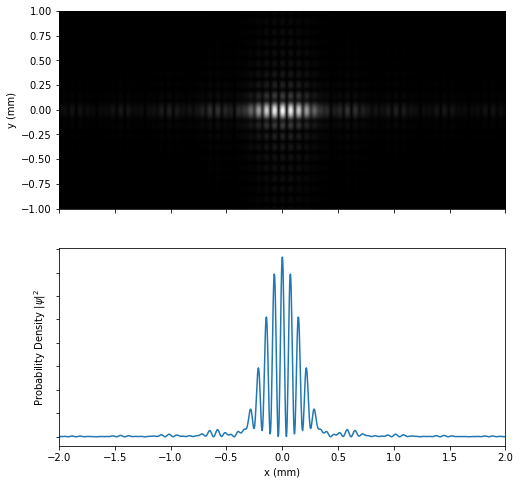
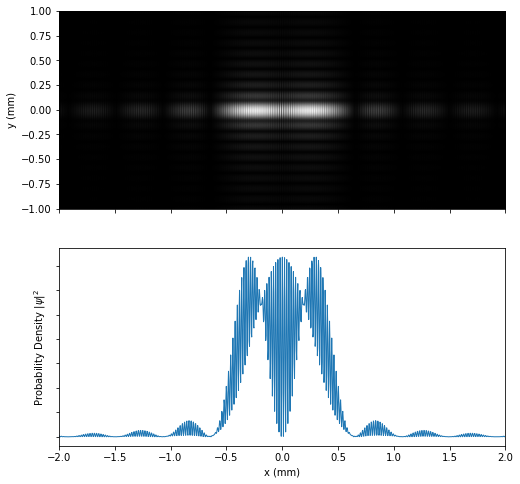
Next we use two slits with the previous dimension, but now their centers are separated by a distance of $0.128 \text{ mm} $. We can see in the following plot that the single slit interference pattern it's the envelope of the double slit interference:
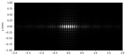
However, this last property will not be fulfilled if the distance between the slits is large enough. To illustrate it, we have represented the interference pattern with the slits separated $0.500 \text{ mm}$:
As can also be seen, the distance between the interferential maximums has decreased. This is because this parameter decreases inversely proportional to the distance between the slits.
In the next post, we´ll describe a more versatile method that allows us to solve the diffraction integral exactly, without recurring to the Fresnel approximation:
Bibliography
[1] Introduction to Fourier Optics J. Goodman sec. 3.5